%matplotlib inline
%reload_ext autoreload
%autoreload 2Predict on rollout grids
import os
import sys

sys.path.append("../../../")

import getpass
import pickle
from pathlib import Path

import contextily as cx
import geopandas as gpd
import matplotlib.pyplot as plt
import numpy as np
import pandas as pd
from sklearn.preprocessing import MinMaxScaler

from povertymapping import nightlights, settings
from povertymapping.dhs import generate_dhs_cluster_level_data
from povertymapping.feature_engineering import (
    categorize_wealth_index,
    generate_features,
)
from povertymapping.iso3 import get_region_name
from povertymapping.rollout_grids import get_region_filtered_bingtile_grids
Model Prediction on Rollout Grids: Vietnam
This notebook is the final step in the rollout and runs the final model to create relative wealth estimations over populated areas within the given country. The model predictions will have a spatial resolution of 2.4km.
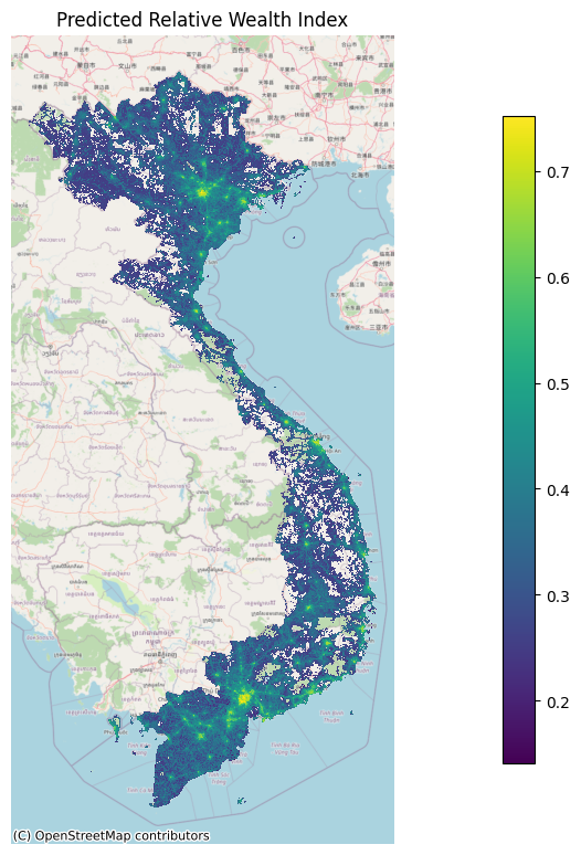
The predicted relative wealth value gives us the relative wealth level of an area compared to the rest of the country, which fixes the value range from 0 (lowest wealth) to 1 (highest wealth). In between these extremes, each area’s wealth estimate is scaled to a value between 0 and 1.
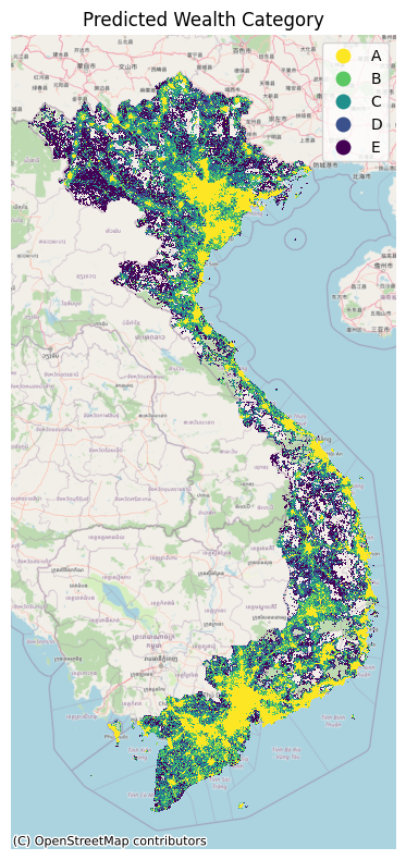
The predicted relative wealth value is later binned into 5 wealth categories A-E by dividing the distribution into quintiles (every 20th percentile).
Set up Data Access
The following cell will prompt you to enter your EOG username and password. See this page to learn how to set-up your EOG account.
# Log-in using EOG credentials
username = os.environ.get("EOG_USER", None)
username = username if username is not None else input("Username?")
password = os.environ.get("EOG_PASSWORD", None)
password = password if password is not None else getpass.getpass("Password?")

# set save_token to True so that access token gets stored in ~/.eog_creds/eog_access_token
access_token = nightlights.get_eog_access_token(username, password, save_token=True)
2023-04-17 15:58:18.815 | INFO | povertymapping.nightlights:get_eog_access_token:42 - Saving access_token to /home/alron/.eog_creds/eog_access_token.txt
2023-04-17 15:58:18.818 | INFO | povertymapping.nightlights:get_eog_access_token:50 - Adding access token to environment var EOG_ACCESS_TOKENSet country-specific parameters
COUNTRY_CODE = "vn"
COUNTRY_OSM = get_region_name(COUNTRY_CODE, code="alpha-2").lower()
OOKLA_YEAR = 2019
NIGHTLIGHTS_YEAR = 2021

rollout_date = "-".join(os.getcwd().split("/")[-2].split("-")[:3])
rollout_grids_path = Path(f"./{rollout_date}-{COUNTRY_CODE}-rollout-grids.geojson")
rollout_grids_pathPath('2023-02-21-vn-rollout-grids.geojson')Set Model Parameters
# Model to use for prediction
MODEL_SAVE_PATH = Path(f"../{rollout_date}-cross-country-model.pkl")
Load Country Rollout AOI
The rollout area of interest is split into 2.4km grid tiles (zoom level 14), matching the areas used during model training. The grids are also filtered to only include populated areas based on Meta’s High Resolution Settlement Layer (HRSL) data.
Refer to the previous notebook 2_vn_generate_grids.ipynb for documentation on generating this grid.
aoi = gpd.read_file(rollout_grids_path)
# aoi.explore() # Uncomment to view data in a map
Generate Features For Rollout AOI
If this is your first time running this notebook for this specific area, expect a long runtime for the following cell as it will download and cache the required datasets. It will then process the relevant features for each area specified. On subsequent runs, the runtime will be much faster as the data is already stored in your filesystem.
%%time
scaler = MinMaxScaler
rollout_aoi = aoi.copy()

# Create features dataframe using generate_features module
features = generate_features(
    rollout_aoi,
    country_osm=COUNTRY_OSM,
    ookla_year=OOKLA_YEAR,
    nightlights_year=NIGHTLIGHTS_YEAR,
    scaled_only=False,
    sklearn_scaler=scaler,
    features_only=True,
    use_aoi_quadkey=True,
)
2023-04-17 15:58:25.434 | INFO | povertymapping.osm:download_osm_country_data:198 - OSM Data: Cached data available for vietnam at /home/alron/.geowrangler/osm/vietnam? False
2023-04-17 15:58:25.435 | INFO | povertymapping.osm:download_osm_country_data:204 - OSM Data: Re-initializing OSM country cache dir at /home/alron/.geowrangler/osm/vietnam...
2023-04-17 15:58:25.436 | INFO | povertymapping.osm:download_osm_country_data:213 - OSM Data: Downloading Geofabrik zip file...
2023-04-17 15:58:25.435 | INFO | povertymapping.osm:download_osm_country_data:204 - OSM Data: Re-initializing OSM country cache dir at /home/alron/.geowrangler/osm/vietnam...
2023-04-17 15:58:25.436 | INFO | povertymapping.osm:download_osm_country_data:213 - OSM Data: Downloading Geofabrik zip file...2023-04-17 16:00:18.898 | INFO | povertymapping.osm:download_osm_country_data:232 - OSM Data: Unzipping the zip file...
2023-04-17 16:00:27.169 | INFO | povertymapping.osm:download_osm_country_data:239 - OSM Data: Successfully downloaded and cached OSM data for vietnam at /home/alron/.geowrangler/osm/vietnam!
2023-04-17 16:00:27.171 | DEBUG | povertymapping.osm:load_pois:160 - OSM POIs for vietnam being loaded from /home/alron/.geowrangler/osm/vietnam/gis_osm_pois_free_1.shp
2023-04-17 16:00:41.992 | INFO | povertymapping.osm:download_osm_country_data:198 - OSM Data: Cached data available for vietnam at /home/alron/.geowrangler/osm/vietnam? True
2023-04-17 16:00:41.992 | DEBUG | povertymapping.osm:load_roads:179 - OSM Roads for vietnam being loaded from /home/alron/.geowrangler/osm/vietnam/gis_osm_roads_free_1.shp
2023-04-17 16:03:17.875 | DEBUG | povertymapping.ookla:load_type_year_data:79 - Contents of data cache: []
2023-04-17 16:03:17.878 | INFO | povertymapping.ookla:load_type_year_data:94 - Cached data available at /home/alron/.geowrangler/ookla/processed/5591b477264360fb7097153cd3331b3d.csv? False
2023-04-17 16:03:17.879 | DEBUG | povertymapping.ookla:load_type_year_data:111 - No cached data found. Processing Ookla data from scratch.
2023-04-17 16:03:18.951 | INFO | povertymapping.ookla:download_ookla_year_data:224 - Ookla Data: Number of available files for fixed and 2019: 4
2023-04-17 16:03:18.953 | INFO | povertymapping.ookla:download_ookla_year_data:237 - Ookla Data: Cached data available for fixed and 2019 at /home/alron/.geowrangler/ookla/fixed/2019? True
2023-04-17 16:03:18.954 | DEBUG | povertymapping.ookla:load_type_year_data:123 - use_quadkey = True. Using columns in quadkey to pull intersecting Ookla data.
2023-04-17 16:03:18.997 | DEBUG | povertymapping.ookla:load_type_year_data:140 - Quadkeys in quadkey are at zoom level 14.
2023-04-17 16:03:18.999 | DEBUG | povertymapping.ookla:load_type_year_data:163 - Ookla data for aoi, fixed 2019 1 being loaded from /home/alron/.geowrangler/ookla/fixed/2019/2019-01-01_performance_fixed_tiles.parquet
2023-04-17 16:03:27.944 | DEBUG | povertymapping.ookla:load_type_year_data:163 - Ookla data for aoi, fixed 2019 2 being loaded from /home/alron/.geowrangler/ookla/fixed/2019/2019-04-01_performance_fixed_tiles.parquet
2023-04-17 16:03:36.147 | DEBUG | povertymapping.ookla:load_type_year_data:163 - Ookla data for aoi, fixed 2019 3 being loaded from /home/alron/.geowrangler/ookla/fixed/2019/2019-07-01_performance_fixed_tiles.parquet
2023-04-17 16:03:46.124 | DEBUG | povertymapping.ookla:load_type_year_data:163 - Ookla data for aoi, fixed 2019 4 being loaded from /home/alron/.geowrangler/ookla/fixed/2019/2019-10-01_performance_fixed_tiles.parquet
2023-04-17 16:03:56.314 | DEBUG | povertymapping.ookla:load_type_year_data:184 - Concatenating quarterly Ookla data for fixed and 2019 into one dataframe
2023-04-17 16:04:08.646 | DEBUG | povertymapping.ookla:load_type_year_data:79 - Contents of data cache: ['5591b477264360fb7097153cd3331b3d']
2023-04-17 16:04:08.647 | INFO | povertymapping.ookla:load_type_year_data:94 - Cached data available at /home/alron/.geowrangler/ookla/processed/67c59b59baa5708f4a8f1f2c1f5a99b9.csv? False
2023-04-17 16:04:08.648 | DEBUG | povertymapping.ookla:load_type_year_data:111 - No cached data found. Processing Ookla data from scratch.
2023-04-17 16:04:08.649 | INFO | povertymapping.ookla:download_ookla_year_data:224 - Ookla Data: Number of available files for mobile and 2019: 4
2023-04-17 16:04:08.650 | INFO | povertymapping.ookla:download_ookla_year_data:237 - Ookla Data: Cached data available for mobile and 2019 at /home/alron/.geowrangler/ookla/mobile/2019? True
2023-04-17 16:04:08.651 | DEBUG | povertymapping.ookla:load_type_year_data:123 - use_quadkey = True. Using columns in quadkey to pull intersecting Ookla data.
2023-04-17 16:04:08.672 | DEBUG | povertymapping.ookla:load_type_year_data:140 - Quadkeys in quadkey are at zoom level 14.
2023-04-17 16:04:08.674 | DEBUG | povertymapping.ookla:load_type_year_data:163 - Ookla data for aoi, mobile 2019 1 being loaded from /home/alron/.geowrangler/ookla/mobile/2019/2019-01-01_performance_mobile_tiles.parquet
2023-04-17 16:04:13.794 | DEBUG | povertymapping.ookla:load_type_year_data:163 - Ookla data for aoi, mobile 2019 2 being loaded from /home/alron/.geowrangler/ookla/mobile/2019/2019-04-01_performance_mobile_tiles.parquet
2023-04-17 16:04:18.913 | DEBUG | povertymapping.ookla:load_type_year_data:163 - Ookla data for aoi, mobile 2019 3 being loaded from /home/alron/.geowrangler/ookla/mobile/2019/2019-07-01_performance_mobile_tiles.parquet
2023-04-17 16:04:25.035 | DEBUG | povertymapping.ookla:load_type_year_data:163 - Ookla data for aoi, mobile 2019 4 being loaded from /home/alron/.geowrangler/ookla/mobile/2019/2019-10-01_performance_mobile_tiles.parquet
2023-04-17 16:04:30.576 | DEBUG | povertymapping.ookla:load_type_year_data:184 - Concatenating quarterly Ookla data for mobile and 2019 into one dataframe
2023-04-17 16:04:38.461 | INFO | povertymapping.nightlights:generate_clipped_raster:376 - Using viirs global file as source raster: /home/alron/.geowrangler/nightlights/global/VNL_v21_npp_2021_global_vcmslcfg_c202205302300.average.dat.tif
2023-04-17 16:04:38.462 | INFO | povertymapping.nightlights:download_url:161 - Using access token from environment var EOG_ACCESS_TOKEN2023-04-17 16:19:58.887 | INFO | povertymapping.nightlights:unzip_eog_gzip:224 - Unzipping /home/alron/.geowrangler/nightlights/global/VNL_v21_npp_2021_global_vcmslcfg_c202205302300.average.dat.tif.gz into /home/alron/.geowrangler/nightlights/global/VNL_v21_npp_2021_global_vcmslcfg_c202205302300.average.dat.tif
2023-04-17 16:21:23.534 | INFO | povertymapping.nightlights:unzip_eog_gzip:235 - Deleting /home/alron/.geowrangler/nightlights/global/VNL_v21_npp_2021_global_vcmslcfg_c202205302300.average.dat.tif.gz
2023-04-17 16:21:23.924 | INFO | povertymapping.nightlights:clip_raster:248 - Generating clipped raster file from /home/alron/.geowrangler/nightlights/global/VNL_v21_npp_2021_global_vcmslcfg_c202205302300.average.dat.tif to /home/alron/.geowrangler/nightlights/clip/d4fabb4208ec7ad172935fe0cff0922d.tif with bounds [102.15087888 8.5592939 109.46777341 23.38259828] and buffer 0.1
2023-04-17 16:21:26.743 | INFO | povertymapping.nightlights:generate_clipped_metadata:421 - Adding metadata.json file /home/alron/.geowrangler/nightlights/clip/d4fabb4208ec7ad172935fe0cff0922d.metadata.jsonCPU times: user 7min 40s, sys: 57 s, total: 8min 37s
Wall time: 25min 18s# Save raw features, can be used for validation
raw_features = features[[col for col in features.columns if "_scaled" not in col]]
# Then keep only scaled columns
features = features[[col for col in features.columns if "_scaled" in col]]Inspect the generated features
features.info()<class 'pandas.core.frame.DataFrame'>
Int64Index: 50880 entries, 0 to 50879
Data columns (total 61 columns):
# Column Non-Null Count Dtype
--- ------ -------------- -----
0 poi_count_scaled 50880 non-null float64
1 atm_count_scaled 50880 non-null float64
2 atm_nearest_scaled 50880 non-null float64
3 bank_count_scaled 50880 non-null float64
4 bank_nearest_scaled 50880 non-null float64
5 bus_station_count_scaled 50880 non-null float64
6 bus_station_nearest_scaled 50880 non-null float64
7 cafe_count_scaled 50880 non-null float64
8 cafe_nearest_scaled 50880 non-null float64
9 charging_station_count_scaled 50880 non-null float64
10 charging_station_nearest_scaled 50880 non-null float64
11 courthouse_count_scaled 50880 non-null float64
12 courthouse_nearest_scaled 50880 non-null float64
13 dentist_count_scaled 50880 non-null float64
14 dentist_nearest_scaled 50880 non-null float64
15 fast_food_count_scaled 50880 non-null float64
16 fast_food_nearest_scaled 50880 non-null float64
17 fire_station_count_scaled 50880 non-null float64
18 fire_station_nearest_scaled 50880 non-null float64
19 food_court_count_scaled 50880 non-null float64
20 food_court_nearest_scaled 50880 non-null float64
21 fuel_count_scaled 50880 non-null float64
22 fuel_nearest_scaled 50880 non-null float64
23 hospital_count_scaled 50880 non-null float64
24 hospital_nearest_scaled 50880 non-null float64
25 library_count_scaled 50880 non-null float64
26 library_nearest_scaled 50880 non-null float64
27 marketplace_count_scaled 50880 non-null float64
28 marketplace_nearest_scaled 50880 non-null float64
29 pharmacy_count_scaled 50880 non-null float64
30 pharmacy_nearest_scaled 50880 non-null float64
31 police_count_scaled 50880 non-null float64
32 police_nearest_scaled 50880 non-null float64
33 post_box_count_scaled 50880 non-null float64
34 post_box_nearest_scaled 50880 non-null float64
35 post_office_count_scaled 50880 non-null float64
36 post_office_nearest_scaled 50880 non-null float64
37 restaurant_count_scaled 50880 non-null float64
38 restaurant_nearest_scaled 50880 non-null float64
39 social_facility_count_scaled 50880 non-null float64
40 social_facility_nearest_scaled 50880 non-null float64
41 supermarket_count_scaled 50880 non-null float64
42 supermarket_nearest_scaled 50880 non-null float64
43 townhall_count_scaled 50880 non-null float64
44 townhall_nearest_scaled 50880 non-null float64
45 road_count_scaled 50880 non-null float64
46 fixed_2019_mean_avg_d_kbps_mean_scaled 50880 non-null float64
47 fixed_2019_mean_avg_u_kbps_mean_scaled 50880 non-null float64
48 fixed_2019_mean_avg_lat_ms_mean_scaled 50880 non-null float64
49 fixed_2019_mean_num_tests_mean_scaled 50880 non-null float64
50 fixed_2019_mean_num_devices_mean_scaled 50880 non-null float64
51 mobile_2019_mean_avg_d_kbps_mean_scaled 50880 non-null float64
52 mobile_2019_mean_avg_u_kbps_mean_scaled 50880 non-null float64
53 mobile_2019_mean_avg_lat_ms_mean_scaled 50880 non-null float64
54 mobile_2019_mean_num_tests_mean_scaled 50880 non-null float64
55 mobile_2019_mean_num_devices_mean_scaled 50880 non-null float64
56 avg_rad_min_scaled 50880 non-null float64
57 avg_rad_max_scaled 50880 non-null float64
58 avg_rad_mean_scaled 50880 non-null float64
59 avg_rad_std_scaled 50880 non-null float64
60 avg_rad_median_scaled 50880 non-null float64
dtypes: float64(61)
memory usage: 26.1 MBRun Model on AOI
Load Model
with open(MODEL_SAVE_PATH, "rb") as f:
    model = pickle.load(f)
Make Predictions
rollout_aoi["Predicted Relative Wealth Index"] = model.predict(features.values)Binning predictions into wealth categories
Afterwards, we label the predicted relative wealth by binning them into 5 categories: A, B, C, D, and E where A is the highest and E is the lowest.
We can create these wealth categories by splitting the output Predicted Relative Wealth Index distribution into 5 equally sized quintiles, i.e. every 20th percentile.
This categorization may be modified to suit the context of the target country.
rollout_aoi["Predicted Wealth Category (quintile)"] = categorize_wealth_index(
    rollout_aoi["Predicted Relative Wealth Index"]
).astype(str)rollout_aoi.info()<class 'geopandas.geodataframe.GeoDataFrame'>
RangeIndex: 50880 entries, 0 to 50879
Data columns (total 10 columns):
# Column Non-Null Count Dtype
--- ------ -------------- -----
0 quadkey 50880 non-null object
1 shapeName 50880 non-null object
2 shapeISO 50880 non-null object
3 shapeID 50880 non-null object
4 shapeGroup 50880 non-null object
5 shapeType 50880 non-null object
6 pop_count 50880 non-null float64
7 geometry 50880 non-null geometry
8 Predicted Relative Wealth Index 50880 non-null float64
9 Predicted Wealth Category (quintile) 50880 non-null object
dtypes: float64(2), geometry(1), object(7)
memory usage: 3.9+ MBrollout_aoi.head(2)| quadkey | shapeName | shapeISO | shapeID | shapeGroup | shapeType | pop_count | geometry | Predicted Relative Wealth Index | Predicted Wealth Category (quintile) | |
|---|---|---|---|---|---|---|---|---|---|---|
| 0 | 13223003120321 | Phu Quoc | None | VNM-ADM2-3_0_0-B967 | VNM | ADM2 | 500.753008 | POLYGON ((103.46924 9.29731, 103.46924 9.31899... | 0.375743 | B |
| 1 | 13223003120320 | Phu Quoc | None | VNM-ADM2-3_0_0-B967 | VNM | ADM2 | 6.106744 | POLYGON ((103.44727 9.29731, 103.44727 9.31899... | 0.283086 | D |
Save output
%%time
rollout_aoi.to_file(
    f"{rollout_date}-{COUNTRY_CODE}-rollout-output.geojson",
    driver="GeoJSON",
    index=False,
)
CPU times: user 10.8 s, sys: 257 ms, total: 11.1 s
Wall time: 11.2 s# Join back raw features and save
rollout_output_with_features = rollout_aoi.join(raw_features).join(features)
rollout_output_with_features.to_file(
f"{rollout_date}-{COUNTRY_CODE}-rollout-output-with-features.geojson",
driver="GeoJSON",
index=False,
)Visualizations
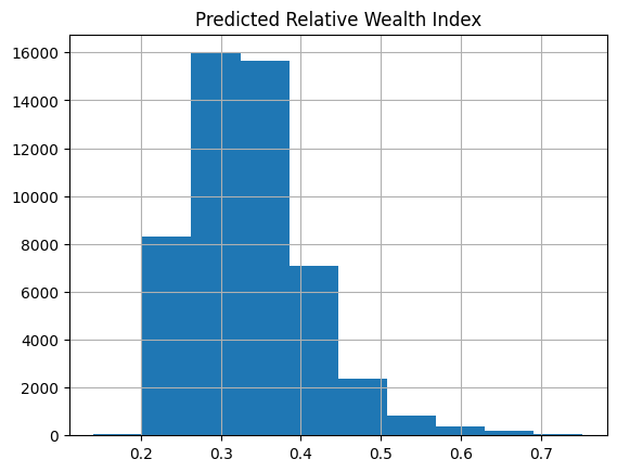
Inspect predicted wealth index and output dataframe
rollout_aoi[["Predicted Relative Wealth Index"]].hist()array([[<AxesSubplot: title={'center': 'Predicted Relative Wealth Index'}>]],
dtype=object)
Create Static Maps
Plot Predicted Relative Wealth Index
plt.cla()
plt.clf()
rollout_aoi_plot = rollout_aoi.to_crs("EPSG:3857")
ax = rollout_aoi_plot.plot(
    "Predicted Relative Wealth Index",
    figsize=(20, 8),
    cmap="viridis",
    legend=True,
    legend_kwds={"shrink": 0.8},
)
cx.add_basemap(ax, source=cx.providers.OpenStreetMap.Mapnik)
ax.set_axis_off()
plt.title("Predicted Relative Wealth Index")
plt.tight_layout()
plt.savefig(f"{rollout_date}-{COUNTRY_CODE}-predicted-wealth-index.png")
plt.show()
<Figure size 640x480 with 0 Axes>
Plot Predicted Relative Wealth Index Category
plt.cla()
plt.clf()
rollout_aoi_plot = rollout_aoi.to_crs("EPSG:3857")
ax = rollout_aoi_plot.plot(
    "Predicted Wealth Category (quintile)",
    figsize=(20, 8),
    cmap="viridis_r",
    legend=True,
)
cx.add_basemap(ax, source=cx.providers.OpenStreetMap.Mapnik)
ax.set_axis_off()
plt.title("Predicted Wealth Category")
plt.tight_layout()
plt.savefig(f"{rollout_date}-{COUNTRY_CODE}-predicted-wealth-bin.png")
plt.show()
<Figure size 640x480 with 0 Axes>
Create an Interactive Map
cols_of_interest = [
    "quadkey",
    "shapeName",
    "shapeGroup",
    "pop_count",
    "avg_rad_mean",
    "mobile_2019_mean_avg_d_kbps_mean",
    "fixed_2019_mean_avg_d_kbps_mean",
    "poi_count",
    "road_count",
    "Predicted Relative Wealth Index",
    "Predicted Wealth Category (quintile)",
]

# Warning: This can be a bit laggy due to the large amount of tiles being visualized

# Uncomment the ff if you want to viz the raw wealth predictions
# rollout_aoi.explore(column='Predicted Relative Wealth Index', tooltip=cols_of_interest, cmap="viridis")

# Uncomment the ff if you want to view the quintiles
# rollout_aoi.explore(column='Predicted Wealth Category (quintile)', tooltip=cols_of_interest, cmap="viridis_r")
Alternatively, you may also try to visualize this interactively in Kepler by uploading the rollout output geojson file.